3D Blood Flow Simulation
Bio-medical researchers have been relying on computational fluid dynamics to model and understand the physical mechanisms behind the formation and progression of hemodynamic disorders. Wall shear stress (WSS) exerted on the walls of the blood vessel due to the flow of blood is one of the main pathogenic factors leading to the development of such disorders.
The magnitude and distribution of the WSS in a blood vessel can provide an insight into the locations of possible aneurysm growth. Moreover, blockages that build up over time can be predicted by having a qualitative understanding of the flow profile.
Computational Fluid Dynamics can be used for modeling and understanding such vital internal flows and insights gained from such studies can help design patient-specific treatments. In this Ansys Fluent tutorial, you will learn how to model three dimensional internal blood flow in a bifurcating artery.
You will create the computational mesh and set up the boundary conditions needed for the simulation. The Non-Newtonian behavior of blood flow will be modeled using the Carreau model.
Moreover, a realistic time-varying boundary condition will be implemented using User Defined Functions (UDF) in order to mimic the pulsatile nature of blood flow.
It serves as an e-learning resource to integrate industry-standard simulation tools into courses and provides a resource for supplementary learning outside the classroom.
The fundamental concepts and the steps needed to successfully model this fluid flow problem are explained using immersive step-by-step walk-through videos. So, let’s get started!
Course Content
- Modeling Objectives & Problem Description – Lesson 1
- Summary of steps for ANSYS Workbench version 19.2
- Pre-Analysis & Start-Up – Lesson 2
- Governing Equations
- Boundary Conditions
- Geometry – Lesson 3
- Mesh – Lesson 4
- Inflation Mesh and Body Sizing
- Named Selection
- Physics Setup – Lesson 5
- Solution Setup
- Boundary Conditions
- Particle Trackin
- Numerical Solution – Lesson 6
- Reference Values
- Numerical Solution
- Numerical Results – Lesson 7
- Load Data from Solution Files
- Plotting Velocity Vectors (3D)
- Adding and Animating Particle Pathlines
- Plotting and Animating Wall Shear on the Artery Wall
- Creating a Sweep for Velocity Profile at Different Sections
- Plot Contours at Specific Locations
- Verification and Validation – Lesson 8
- Mass conservation and Inlet boundary conditions
- Mesh Refinement and Smaller Time-step
- Validation
- References – Lesson 9
- Exercise – Lesson 10
- Adding Obstructions to the Original Artery Geometry
- Adding Stent to the Original Artery Geometry
- Simulating the Non-Newtonian Fluid Using Casson Fluid Model
Lesson 1: Modeling Objectives & Problem Description
Learning Goals
In this tutorial, you will learn to:
- Create a mesh for a three-dimensional internal flow.
- Apply Non-Newtonian fluid properties using the Carreau model.
- Apply time-varying boundary conditions using User Defined Functions (UDF).
Problem Specification
Consider the following 3D model of a carotid artery bifurcation.
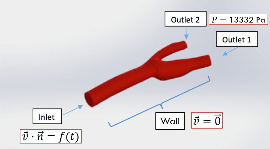
This model is created from a luminal casting of a carotid artery bifurcation and generously shared in Grabcad community.
Blood flows through the bifurcating artery from the inlet (to the left in the graph above) and exits from the two outlets (to the right). The diameter of the artery at the inlet is around 6.3 mm. The diameter of outlet 1 is around 4.5 mm and the diameter of outlet 2 is around 3.0 mm.
The density of blood is 1060 kg/m3 [1]. As blood is a non-newtonian fluid, the coefficient of viscosity of blood is not a constant, but rather, it is a function of velocity gradients.
Here we use the Carreau-model to model blood’s viscosity. Since blood flow is pulsatile and cyclic, the velocity profile at the inlet is a function of time. The pressure at the outlet is defined to be constant (100 mm Hg). More details on boundary conditions will be provided in the next lesson “Pre-Analysis and Set-up”.
The summary of steps for ANSYS Workbench version 19.2 can be found below.
Lesson 2: Pre-Analysis & Start-Up
Pre-Analysis
In the Pre-Analysis step, we’ll review the following:
- Governing Equations: We will review the governing equations that need to be solved in this problem.
- Boundary Conditions: We will go into more details about the boundary conditions that are applied in this problem.
Governing Equations
Before starting a CFD simulation, it is always good to take a look at the governing equations underlying the physics. In this case, although we have additional complexities such as pulsatile flow and non-Newtonian fluids, the governing equations are the same as any other fluids problem.
The most fundamental governing equations are the continuity equation and the Navier-Stokes equations. Here, let’s have a quick review of the equations.
Continuity Equation:
![]()
However, as blood can be regarded as an incompressible fluid, the rate of density change is zero, thus the continuity equation above can be further simplified in the form below:
![]()
The Navier-Stokes Equation:
![]()
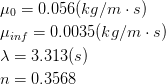
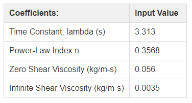
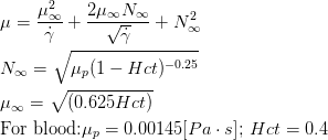
One thing to notice in the Navier-Stokes equation is that the viscosity coefficient of μ is not a constant but rather a function of shear rate. Blood gets less viscous as the shear rate increases (shear thinning). Here, we model the blood viscosity using the Carreau fluids model. The mathematical formulation of the Carreau model is as follows:
![]()
In the equations above, μeff is the effective viscosity. μ0 , μinf , λ, and n are material coefficients.
For the case of blood [2],
Boundary Conditions
Wall:
The easiest boundary condition to determine is the artery wall. We simply need to define the wall regions of this model and set it to “wall”. From a physical viewpoint, the “wall” condition dictates that the velocity at the wall is zero.
Inlet:
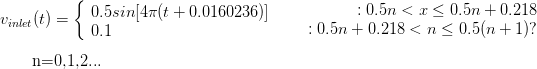
As we know, mammalian blood flow is pulsatile and cyclic in nature. Thus the velocity at the inlet is not set to be a constant, but instead, in this case, it is a time-varying periodic profile. The pulsatile profile within each period is considered to be a combination of two phases. During the systolic phase, the velocity at the inlet varies in a sinusoidal pattern.
The sine wave during the systolic phase has a peak velocity of 0.5 m/s and a minimum velocity of 0.1 m/s. Assuming a heartbeat rate of 120 per minute, the duration of each period is 0.5 s. This model for pulsatile blood flow is proposed by Sinnott et, al. [3] A figure of the profile within two periods is given below:
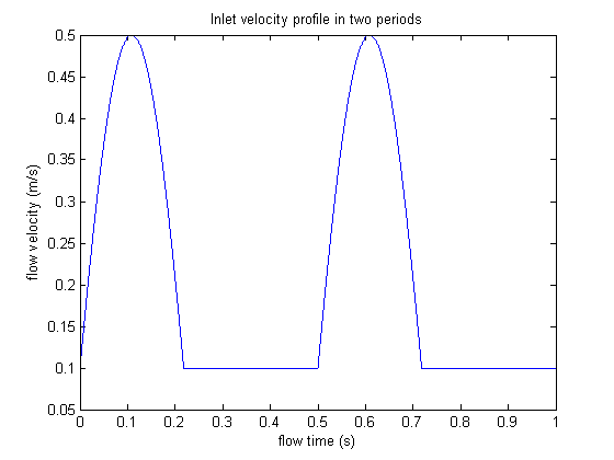
To describe the profile more clearly, a mathematical description is also given below:
Outlets:
The systolic pressure of a healthy human is around 120 mm Hg and the diastolic pressure of a healthy human is around 80 mm Hg. Thus, taking the average pressure of the two phases, we use 100 mm Hg (around 13332 Pascal) as the static gauge pressure at the outlets.
Lesson 3: Geometry
The geometry is given in STEP format. Click HERE (Step File) to download it. The following video shows you how to import the geometry file into Ansys SpaceClaim.
Note the areas of the inlet and outlets, compare to those in the book.
Make sure to save the project!
Lesson 4: Mesh
This lesson will show you how to create the mesh for the fluid domain and create Named Selections.
Inflation Mesh and Body Sizing
In the video, we will learn the following:
- creating an inflation mesh on the walls, and
- using a body sizing to generate the mesh
Named Selection
In this video, we will be creating the necessary ‘Named Selections’ for the meshed object in Ansys Meshing.
Lesson 5: Physics Setup
In this lesson, we will set up the simulation type, materials and the boundary conditions needed to perform the simulation. We will also setup particle tracking so that we can create particle trajectories later on.
Solution Setup
Watch the following video for setting up the Ansys Fluent model to solve for the flow field in the bifurcating artery.
Summary for the video:
- General → Change from “steady” to “transient”
- Materials → Fluid → Change “Name” to “Blood” → Change “Density” to 1060 kg/m3 → Select “Carreau” for Viscosity (NOTE: Carreau Model is active only in Laminar flow)
Details for Carreau Model:
Boundary Conditions
Click HERE to download a zipped file containing the User Defined Function (UDF) used in this tutorial.
Watch the following video for demonstrations:
Summary for the video:
- UDF: Define → User Defined → Functions → Interpreted.
- Boundary Conditions → Inlet → Velocity Inlet → Edit → Velocity Magnitude → Change “Constant” to “udf inlet_velocity”.
- Outlet1 → Pressure Outlet → Edit → Gauge Pressure 13332.
- Outlet2 same as outlet1.
For ANSYS 19.2, follow the steps below
- User Defined →Functions →Interpreted
- Add UDF file vinlet_udf.c → Build →Read
- Boundary Conditions → Inlet → Velocity Inlet → Edit → Velocity Magnitude → Change “Constant” to “udf inlet_velocity”.
- Outlet1 → Pressure Outlet → Edit → Gauge Pressure 13332
- Outlet2 same as outlet1
Particle Tracking
The motivation for tracking the particles here is to setup for creating particle trajectories later on.
Watch the following video for demonstrations:
Summary for the video:
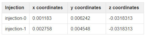
- Define → Injections → Create → Change “Particle Type” to Massless → Input the coordinates (see the table below)
- Repeat the steps above to inject another particle (or more, if you like)
For ANSYS 19.2, follow the steps below
- Setting Up Physics → Model Specific → Discrete Phase Models>Injections
- Injections → Create → Change “Particle Type” to Massless → Input the coordinates (see the table below)
- Repeat the steps above to inject another particle
Summary of coordinates for example injections:
Lesson 6: Numerical Solution
In this lesson, we will learn how we can specify the reference entities that are used by Ansys Fluent for calculating non-dimensionalization. We will then learn how we can setup solution monitors for monitoring Drag and set up calculation activities to export solution data for post-processing later on.
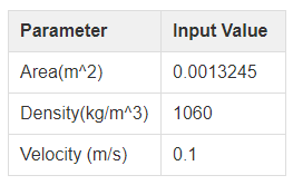
Reference Values
The drag is calculated by integrating the shear and pressure at the wall. The drag coefficient is then calculated by non-dimensionalizing the drag. The reference entities used in the non-dimensionalization are defined in the Reference Values panel in Fluent.
Note that the “Reference Values” will not change your solution for the velocity and pressure at the cell centers. It will affect only the drag coefficient and any other non-dimensional quantities calculated from the solution. Watch the following video for demonstrations:
If you have used SpaceClaim to create geometry, refer to the steps below for Total Surface Area
- Open Spaceclaim → Measure → Mass Properties
- Note down Total Surface Area
Summary of Reference Values:
Numerical Solution
Watch the following video for demonstrations:
Summary for the video:
- Monitors → Create → Drag → Print to Console → wall_artery
- Solution Initialization → Hybrid Initialization → Initialize
- Calculation activities → Create → Solution Data Export → Change File Type to “CFD-Post Compatible”
Quantities for export: Static Pressure, Total Pressure, Velocity Magnitude, x velocity, y velocity, z velocity, Wall Shear (* note that you need to export all three components of velocity in order to plot vector field in CFD-Post!) - Create → Particle History Export → File Type to CFD-Post → Select the injections → Choose to save directory
- Run Calculation → Time Step Size 0.01 → Number of time steps 50 → Max Iterations/time step 200 → Hit “Calculate”!
If you are using ANSYS 19.2, refer to the steps below:
- Setup → Reference values → Type in the values given in the above table
- Report Monitors → New → Force Report → Drag → wall artery
- Solution Initialization → Hybrid Initialization → Initialize
- Calculation Activities → Create → Solution Data Export
- Change the file type to “CDAT for CFD Post and Ensight”
- Select above-mentioned quantities for export
- Calculation Activities → Create → Particle Data History Export → Select both injections
- Run Calculation → Time Step Size(s) 0.01 → Number of Time Steps 50 → Maximum Iterations/Time Step 200 → Hit Calculate
Before running the calculation, you should also create a monitor for the inlet velocity so that we can check that the UDF is working correctly in the Verification and Validation step.
- Report Monitors → New → Surface Report → Area-weighted Average
- Set Field Variable as Velocity → Velocity Magnitude
- Select “inlet” under Surfaces
- Make sure to check the box next to Report Plot
- Give it a suitable name and click OK
Lesson 7: Numerical Results
In this lesson, we will post-process the numerical results generated in the previous step and analyze the flow field. We will start by loading the saved data and plotting velocity vectors in 3D space.
We will then add particle pathlines and animate them to visualize the flow. We will also plot and animate the shear stresses experienced by the arterial walls due to the pulsatile blood flow. Lastly, we will create a sweep of velocity profiles at different cross-sections.
Load Data from Solution Files
Watch the following video for demonstrations:
Summary of the video:
- Return to Workbench → Component Systems → Results(Drag into Project Schematic) → Open Results
- Click on import data button → Load complete history as → “a single case”
Plotting Velocity Vectors (3D)
Watch the following video for demonstrations:
Summary of the above video:
-
- Right click on wall_artery → Edit
- Click on the Render → Transparency 0.7
- On the top toolbar, click on the vector icon
- Name it Velocity Vector
- For the Location in the Geometry tab, select fluid_zone
- Click Apply
Adding and Animating Particle Pathlines
Watch the following video for demonstrations:
The particle track file can be downloaded at this link.
Summary of the above video:
- Turn off Velocity Vector by unchecking the box next to Velocity Vector
- Go to File → Import → Import FLUENT Particle Track File
- Browse for part
- Double click on the particle track
- Go to Color tab
- For Variable, choose Velocity
- Apply
- Go to Symbol tab
- Check the box Show Symbols
- For Max Time is, choose Current Time
- For Scale, type 0.5
- Apply
- To animate this particle, click on the Animation icon next to the clock icon
- Click FLUENT PT for massless
- Press play to preview
- To save video, check box Save Movie
- Choose the speed of the video you want to playback
- To start the animation that will be saved, press play
- When you reach your desired time, press stop
Plotting and Animating Wall Shear on the Artery Wall
Watch the following video for demonstrations:
Summary of the above video:
- Double click on FLUENT PT for Massless to turn it off
- Click on Location → select Surface Group
- Name it Artery Wall
- Under Geometry tab, choose wall_artery
- Under the Color tab, choose Variable Wall Shear
- Apply
- To animate, click on the Animation icon
- Repeat the process from the previous tutorial to produce a video
Creating a Sweep for Velocity Profile at Different Sections
Watch the following video for demonstrations:
Summary of the above video:
- Turn off artery_wall
- Click on Location → select Isosurface
- Name it XY Plane
- Under Geometry tab, choose Variable Z
- For Value, drag the slider to the most left smallest value
- Under Color tab, change Mode to Variable
- For Variable, choose Velocity
- Apply
- Click on Animation Icon
- Click on XY Plane for animation
- Repeat process from previous tutorial videos
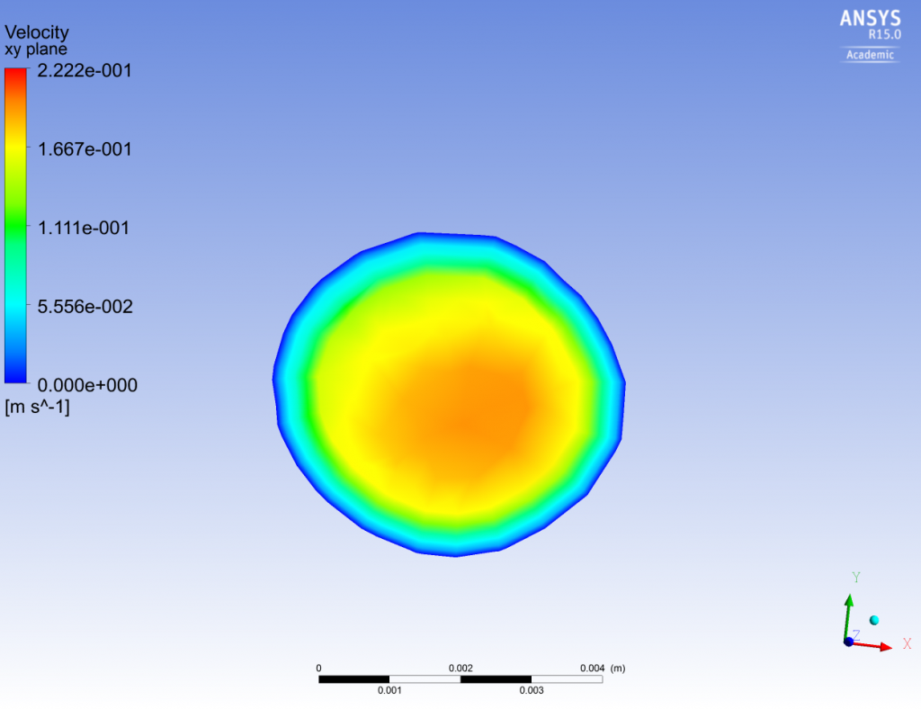
Plot Contours at Specific Locations
Basically, you need to first create a plane, and then color the plane by your desired variable. Methods to create a plane include:
Plane (you can specify three point, or one point and a normal vector), Isosurface (where you can specify x, y or z values), user surface or surface group. After constructing your surface, color it by variable, and choose the variable you would like to plot.
Finally, you may toggle your view to face normal to the plane, and then turn of all the 3D faces and wireframe that might disturb your view. Then you can take a snapshot of the contour. Example given below:
Isosurface → variable z → Color by velocity → turn off the walls and outlets and wireframe
Lesson 8: Verification and Validation
The two things we will check for verification are the mass conservation and inlet boundary conditions. We will check the inlet boundary conditions to ensure that the UDF is doing what we expected it to.
Then, we will do a mesh refinement and use a smaller time-step to check whether the results are consistent with the original calculation. By using a finer mesh and a smaller time-step, we will investigate the effects of truncation error caused by spatial discretization and temporal discretization.
Then we will do a case comparison for the results obtained after spatial and temporal refinement.
Mass conservation and Inlet boundary conditions
To check whether mass is conserved in this calculation, open up solutions. Go to Reports → Fluxes and then under options, check “Mass flow rate”. Then select the one inlet and two outlets.
We would expect the mass flux to sum up to zero (or extremely small).
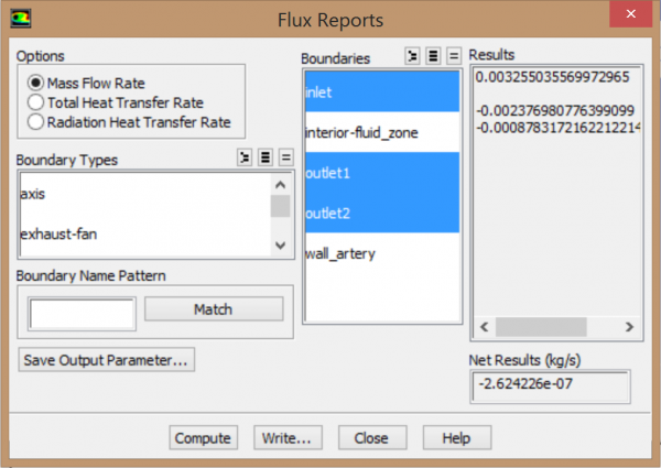
As we can see from the window above, the mass fluxes add up to -2.624226e-07, which is very close to zero.
Inlet boundary conditions are checked during the calculations. As long as the surface monitor for average velocity has been turned on, the velocity at the inlet will be plotted. Below is the velocity profile at the inlet plotted during the calculation.
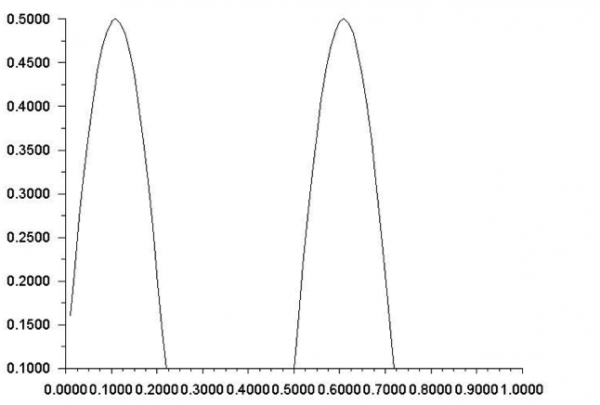
The profile matches our mathematical function for inlet velocity perfectly.
Mesh Refinement and Smaller Time-step
In the original calculation, a body sizing of 1e-3 is applied, hence the total number of cells in that mesh is 145082. However, in the refined mesh, a body sizing of 5e-4, which is half of the original size, is applied, and resultantly the total number of cells in the refined mesh is 217475.
Ideally, it is also good to refine the inflation mesh by choosing a smaller inflation thickness. In this tutorial, this has not been done, but readers are encouraged to do this step.
In the original calculation, the time-step that was used was 0.01 s. For verification, a smaller time-step of 0.005 s is used.
Case Comparison
After recalculating the cases, a case comparison is made to check the differences. First, the wall shear on the artery wall is plotted for comparison.
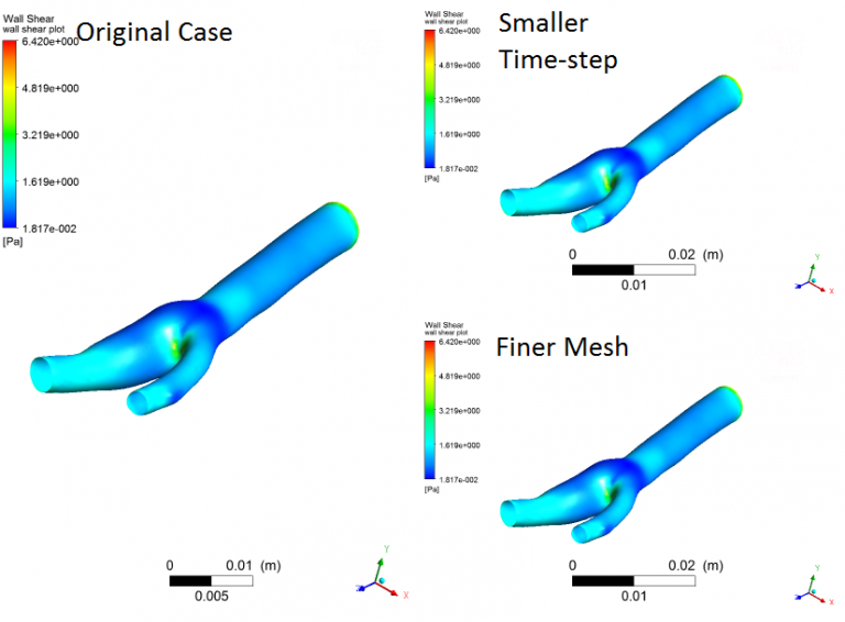
From the plot above, we can tell that the wall shear distribution is almost identical throughout all three cases. But in order to make a more mathematically rigorous comparison, we need to extract some numerical data from the cases for comparison. The function calculator can be used to extract numerical information from the cases.
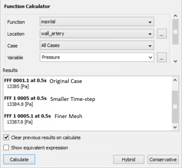
Here in the example, the maximum pressure on the wall in the three cases is calculated. By comparing the values, we can see that the difference between the original case and the refined cases is only 0.02% and 0.001%. This shows that pressure value is consistent in all cases.
Thus based on these results from case comparisons, it is safe to say that the results obtained in the original case are verified.
Validation
In this blood flow in 3D bifurcating artery simulation, we have included most of the physical properties, such as the non-newtonian fluid properties of blood and the pulsatile nature of the flow.
However, in order to perform a simulation closer to the real scenario, elastic wall features should be included. This can be done by coupling the solution from FEA simulation and CFD simulation in Ansys Workbench.
It is also always good to compare the results obtained from simulations with experimental results. In this case, however, we do not have experimental data based on the exact same geometry.
Lesson 9: References
References:
- Cutnell, John & Johnson, Kenneth. Physics, Fourth Edition. Wiley, 1998: 308.
- Siebert, Mark W. & Fodor, Petru S. Newtonian and Non-Newtonian Blood Flow over a Backward- Facing Step – A Case Study. Excerpt from the Proceedings of the COMSOL Conference 2009 Boston 2009.
- SINNOTT, Matthew. CLEARY, Paul W. & PRAKASH, Mahesh. An investigation of pulsatile blood flow in a bifurcating artery using a grid-free method. Fifth International Conference on CFD in the Process Industries CSIRO, Melbourne, Australia 2006
Acknowledgement:
This tutorial is made under great help and support from Dr. Rajash Bhaskaran, Cornell University.
Lesson 10: Exercise
As an exercise, we will add more complexity to the simulation that pertains to a more realistic problem. We will first see how we can add obstruction to the original artery geometry.
These can be thought of as blockages that build up over time. Next, we will learn how we can add a stent to the original artery geometry. Lastly, we will see how we can implement a Casson fluid model using a User Defined Function (UDF) in Ansys Fluent.
Adding Obstructions to the Original Artery Geometry
Watch the following video for a demonstration of how to add obstructions to the original artery geometry using Ansys SpaceClaim.
Quick Summary:
- Edit Model in SpaceClaim
- File → SpaceClaim Options → Set Minimum Grid Spacing to 0.1mm
- Place a point where you want the centroid of the obstruction located
- Merge the surrounding faces using Repair → Merge Faces
- Hide Artery
- Sketch an ellipse on XZ plane
- Major axis length (along Z): 12mm
- Minor axis length (along X): 4mm
- Pull → Select the Z axis → Click the → button
- Move → Up to → Click on the Point from earlier
- Unhide Artery and make sure ellipsoid is properly sized and positioned
- Use Pull → Scale to resize the ellipsoid
- Use Move to reposition the ellipsoid using the directional or orientational handles
- Click Combine
- Click the artery, then the ellipsoid (should result in three solids)
- Delete or suppress all entities except the artery
- Click Pull, click on the edge of the resulting depression and create a fillet
- If you need to restart for any reason, simply CTRL + click the depression and the fillet and then click Fill (make sure you click the green checkmark that is on the screen)
Adding Stent to the Original Artery Geometry
Watch the following video for a demonstration of how to add a stent to the original artery geometry using Ansys SpaceClaim.
You will need to suppress the solid created to generate the effect of the stent before opening the geometry in the mesher.
Quick Summary:
- Create a new sketch, move to one end of the obstruction
- Use Spline to mimic the artery boundary (just click on the edge of the artery that is visible and follow the dots that show up)
- Use Offset Curve to create two more curves: one inside and one outside the artery
- Return to 3D mode
- Hide the artery
- Delete the inner portions of the resulting surfaces leaving only the outer ring
- Unhide the artery
- Do the same on the other end of the obstruction
- Hide the artery
- Use Blend and then control + click the two faces that remain
- Unhide the artery
- Ctrl + Click the missing ellipse and fillet and click Fill if you haven’t already
- Use Combine as before to create three solids
- Delete or suppress all entities except the artery
- Use pull to smooth any sharp edges as desired
Simulating the Non-Newtonian Fluid Using Casson Fluid Model
A user defined function (UDF) can be used to implement the Casson fluid model. The Casson fluid model is given below:
A UDF incorporating the equations above is included in the file that you can download here. This file also contains the UDF for defining the time variation of the inlet velocity.
You need to use this file for the Casson model and not the one provided in the tutorial. This is necessary because all UDF’s need to be in one .c file. You could also use this .c file for all your cases whether you are using the Casson model or not.
In order to implement this file in Fluent, in the top menu bar, under “Define” → “User Defined” → “Functions”, choose “Interpreted”. Find the .c file in the directory, and choose “Interpret”.
Then under materials, double click on the fluid you defined, and for viscosity, choose “User Defined”. Then choose “casson_viscosity”. You assign the inlet velocity as in the tutorial.
This tutorial was prepared by Ansys Innovation Courses.
0 Comments